Rounding data and dynamic programming
有些 NP-hard problem 在 input data 以 unaray 的形式表达时,可以使用 dynamic programming 在以 input size 为自变量的 polynomial time 解决,此时的 algorithm 被称为是 pseudopolynomial1 的。通过 rounding input value 可以得到一个 polynomial in the input size 的 approximation algorithm.
对于其他 problem, 则通常将 input instance 分为 "large" 和 "small" 两个部分,对 large input 进行 rounding, 然后使用 DP 在 polynomial-time 单独求解得到一个存在 error parameter 的 solution, 再通过一些方式结合 small input 得到最终的 solution.
The knapsack problem
给定 item 的集合 \(I = \{1, \dots, n\}\), 每个 item 有 value \(v_{i}\) 与 size \(s_{i}\), 所有 value 与 size 都是正整数。knapsack 的容量为 \(B\), 也是一个正整数。要求出 item 的子集 \(S \subseteq I\), 满足 \(\sum_{i \in S}s_{i} \leq B\), 使得 \(\sum_{i \in S}v_{i}\) 最大。
经典的 DP 算法如下:
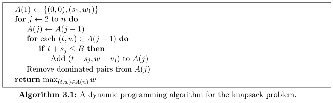
Theorem 3.1
Algorithm 3.1 correctly computes the optimal value of the knapsack problem.
Algorithm 3.1 的时间复杂度为 \(O(n \min(B, V))\), 其中 \(V =\sum_{i \in I}v_{i}\). 若所有 input 都用 binary 编码,此时 input \(B\) 的 size 为 \(\log_{2} B\), \(O(nB)=O\left(n 2^{\log_{2}B}\right)\) 为 input number \(B\) 的 exponential, 因此并不是 polynomial in input size.
Definition 3.2
An algorithm for a problem \(\Pi\) is said to be pseudopolynomial if its running time is polynomial in the size of of the input when the numneric part of the input is encoded in unary.
若 \(V\) 是 \(n\) 的 polynomial, 那么 \(O(n \min(B, V))\) 就会是 \(n\) 的 polynomial. 我们可以通过将 \(v_{i}\) round 到 \(n\) 的 polynomial 来得到一个真正的 polynomial-time (但是 approximation) algorithm, 合适的 rounding 技巧可以使结果的误差较小。
Definition 3.3
A polynomial-time approximation scheme (PTAS) is a family of algorithms \(\{A_{\epsilon}\}\), where there is an algorithm for each \(\epsilon > 0\), such that \(A_{\epsilon}\) is a \((1 + \epsilon)\)-approximation algorithm (for minimization problems) or a \((1 - \epsilon)\)-approximation algorithm (for maximization problems).
\(A_{\epsilon}\) 的 running time 会取决于 \(1 / \epsilon\), 一般考虑在 \(1 / \epsilon\) 上有较好的 bound 的 algorithm:
Definition 3.4
A fully polynomial-time approximation scheme (FPAS, FPTAS) is an approximation scheme such that the running time of \(A_{\epsilon}\) is bounded by a polynomial in \(1 / \epsilon\).
下面给出一个 knapsack problem 的 FPAS. 考虑用一个与 \(n\) 有关 (polynomial in \(n\)) 的数 \(\mu\) 来估计 \(v_{i}\), 将 \(v_{i}\) round 到 \(v_{i}'=\lfloor v_{i} / \mu \rfloor\), 然后跑 Algorithm 3.1 得到 item 集合 \(S'\), 最终算法得到的解即为 \(\sum_{i \in S'}v_{i}\).
缩放因子 \(\mu\) 的设计需要满足两点:
- 误差控制:算法是 \((1-\epsilon)\)-approximation, 因此总误差不能超过 \(\epsilon \mathrm{OPT}\)
- 计算效率:缩放后的价值范围足够小,使动态规划复杂度可以接受
记最优解得到的 item 集合为 \(S\), 则 \(\mu\sum_{i \in S}v_{i}' \geq \mathrm{OPT}-n\mu\), 由于 \(S'\) 为此时的最优解,因此有 \(\mu \sum_{i \in S'}v_{i}' \geq \mu \sum_{i \in S}v_{i}' \geq \mathrm{OPT} - n \mu\), 又 \(\mu \cdot \sum_{i \in S'}v_{i}' \leq \sum_{i \in S'}v_{i}\), 于是总误差上界为 \(n \mu\).
记 \(M = \max_{i \in I}v_{i}\), 则显然有 \(\mathrm{OPT} \geq M\), 不妨令 \(n \mu = \epsilon M\) 控制误差恒不超过 \(\epsilon\) 倍 \(\mathrm{OPT}\) 的下界, 得到 \(\mu = \epsilon M / n\), 于是 \(v_{i}' = \lfloor \frac{v_{i}}{\epsilon M / n} \rfloor\).

此时有 \(V'=\sum_{i=1}^n v_{i}' = \sum_{i=1}^n \lfloor \frac{v_{i}}{\epsilon M / n} \rfloor = O(n^2 / \epsilon)\), 算法的时间复杂度为 \(O(n \min(B, V')) = O(n^{3} / \epsilon)\), 满足 bounded by a polynomial in \(1 / \epsilon\).
Theorem 3.5
Algorithm 3.2 is a fully polynomial-time approximation scheme for the knapsack problem.
\(\textit{Proof}.\) 只需证明算法是 \((1-\epsilon)\)-approximation 即可。通过下列不等式可以证明:
Scheduling jobs on identical parallel machines
不难想到将 job 分为 short job 和 long job, 然后对数量被限制到常数级别的 long job 求出 optimal schedule, 再将 short job 按照 list scheduling 加入当前 schedule 中。
具体来说,将 \(p_{i} \geq \frac{1}{km} \sum_{i=1}^{n} p_{i}\)2 的 job 视为 long job, 则 long job 至多有 \(km\) 个,其中 \(k\) 为常数,若假定 \(m\) 也是常数,那么 long job 的数量也是常数级别,此时可以直接暴力求出 optimal schedule for long jobs, 总的状态数为 \(O(m^{km})\) 为常数,然后对 short jobs 从大到小排序后按照 list scheduling 加入 schedule 得到最终的 schedule, 最后的时间复杂度为 \(O(n\log n + m^{km})=O(n\log n)\), 瓶颈在于排序,显然属于 polynomial-time algorithm. 记此类算法为 \(\{ A_{k} \}\).
在上一章中 list scheduling 算法有结论
其中 \(\ell\) 为最晚完成的 job. 对于 \(A_{k}\) 得到的 schedule, 若最晚完成的 job 是 long job, 那么此时的 \(C_{\max}=C_{\max}^{\ast}\); 若最晚完成的 job 是 short job, 根据结论有
令 \(\epsilon=\frac{1}{k}\), 则 \(A_{k}\) 是 \((1+\epsilon)\)-approximation polynomial-time algorithm.
Theorem 3.6
The family of algorithms \(\{ A_{k} \}\) is a polynomial-time approximation scheme for the problem of minimizing the makespan on any constant number of identical parallel machines.
如果只在最晚完成的 job 是 long job 时才对 long job 计算 optimal schedule, 否则沿用 knapsack 的 DP 方法计算一个非最优的 schedule, 这样可以移除 \(m\) 是常数的限制。
由于 \(C_{\max}^{\ast}\) 未知,不妨设 target length 为 \(T\), 令 \(p_{j} \geq T / k\) 的 job 为 long job, 若设置的 \(T \geq C_{\max}^{\ast}\), 此时 long job 的数量相对少,可以利用 DP 在 poly-time 得到一个关于 \(T\) 的近似解,然后便可调小 \(T\) 值;若设置的 \(T < C_{\max}^{\ast}\), 此时 long job 的数量较多,poly-time 内难以找到与 \(T\) 相关的近似解,因此可以 return false 并调大 \(T\) 值,最终会得到一个 \(\leq C_{\max}^{\ast}\) 的 \(T\) 值并由此计算出一个近似解,最后再利用 list scheduling 加入 short job 即可。
记上述算法为 \(\{ B_{k} \}\), 具体过程如下:将 long job 的 length round 到最近的 \(T / k^{2}\) 的倍数 \(i \cdot T / k^{2}\), 之后只需要关心 \(i\) 而不是 \(p_{j}\). 在 target length 为 \(T\) 的设定下,每个 machine 会被分配的 job 至多 \(T / \frac{T}{k} = k\) 个,并且最大的 job 满足 \(p_{j} \leq T\) (否则必然有 \(T < C_{\max}^{\ast}\)), 因此按照 \(i\) 分类的话 long job 至多可以分为 \(T / \frac{T}{k^{2}} = k^{2}\) 类,于是每个 machine 的状态可以用一个 \(k^{2}\) 维的 vector \((s_{1}, s_{2}, \dots, s_{k^{2}})\) 表示,当满足下列不等式时称它为 machine configuration:
记所有 machine conofiguration 构成的集合为 \(\mathcal{C}\), 则 \(\lvert \mathcal{C} \rvert \leq (k+1)^{k^{2}}\), 为常数级别。
然后 DP (类似分组背包) 的状态方程为
可以在 \(O(m \cdot \lvert \mathcal{C} \rvert)\) 时间内求出 round 后的最优解。由于限定了单个 machine 的 load \(\leq T\), 设该解在任意 machine 上分配的 job 集合为 \(S\), 有 \(\lvert S \rvert \leq k\), 且单个 job 满足 \(p_{j} - p_{j}' \leq T / k^{2}\), 所以有
于是 DP 的近似解满足 \(C_{\max}' \leq \left( 1 + \frac{1}{k} \right)T\), 且如果 \(T < C_{\max}^{\ast}\) 就无法找到合法的解,最后加上 short job 不难证明在最后完成的 job 是 short job 时,由于 \(\sum_{j=1}^{n}p_{j} / m \leq T\), 于是
因此,\(\{ B_{k} \}\) 会在 poly-time 内要么返回 \(T\) 无解要么返回 \(C_{\max} \leq \left( 1 + \frac{1}{k} \right)T\) 的解。
设
作为 \(T\) 的上下界然后二分即可,最后得到的 \(T \leq C_{\max}^{\ast}\), 因此 \(\{ B_{k} \}\) 可以给出 \(C_{\max} \leq \left( 1 + \frac{1}{k} \right)C_{\max}^{\ast}\) 的解,再令 \(\epsilon = \frac{1}{k}\), 于是 \(\{ B_{k} \}\) 为 \((1 + \epsilon)\)-approximation poly-time algorithm.
Theorem 3.7
There is a polynomial-time approximation scheme for the problem of minimizing the makespan on an input number of identical parallel machines.
由于 DP 的状态数为 \(O\left((k+1)^{k^{2}}\right)\), 即 exponential in \(O\left(1 / \epsilon^{2}\right)\), 因此 \(\{ B_{k} \}\) 并不是 FPAS.
事实上,这个 scheduling problem 是 strongly NP-complete 的:即使将每个 job 的 processing time 限制为 \(q(n)\), 在这个特殊情况下也依旧是 NP-complete 的。若存在解决该 scheduling problem 的 FPTAS, 那么就可以令 \(k=\lceil 2nq(n) \rceil \geq 2nP\), 其中 \(P = \max_{j=1, \dots, n}p_{j}\), 于是算法的解满足 \(C_{\max} \leq \left( 1 + \frac{1}{k} \right)C_{\max}^{\ast} \leq C_{\max}^{\ast} + \frac{1}{2}\), 由于 \(C_{\max}, C_{\max}^{\ast}\) 为整数,因此 \(C_{\max} = C_{\max}^{\ast}\), 从而存在算法在 poly-time 解决 processing time 被限制为 \(q(n)\) 的 scheduling problem, 从而可以推出 \(\mathrm{P=NP}\).
一个更 general 的结论是:对于任意优化问题,若该问题是 strongly NP-complete 的,那么它不存在 FPAS.
The bin-packing problem
bin-packing problem 指的是下列问题:
给定 \(n\) 个大小分别为 \(a_{1}, a_{2}, \dots, a_{n}\) 的 pieces (或 items), 满足
\[1 > a_{1} \geq a_{2} \geq \cdots \geq a_{n} > 0;\]我们希望将这些 pieces 装进尽可能少的 bins, 其中每个 bin 的容量为 1.
bin-packing problem 的特殊情形下可以转化为 partition problem: 给定 \(n\) 个正整数 \(b_{1}, \dots, b_{n}\) 满足 \(B=\sum_{i=1}^n b_{i}\) 为偶数,问能否将下标集合 \(\{ 1,\dots,n \}\) 划分为集合 \(S\) 和 \(T\) 使得 \(\sum_{i \in S}b_{i} = \sum_{i \in T}b_{i}\).
只需令 \(a_{i}=2b_{i} / B\) 并检查能否装进 2 个 bin 即可将 bin-packing problem 转化为 partition problem. 由于 partition problem 是 NP-complete 的,于是有下列 theorem.
Theorem 3.8
Unless \(\mathrm{P=NP}\), there cannot exist a \(\rho\)-approximation algorithm for the bin-packing problem for any \(\rho < 3 / 2\).
记 \(\mathrm{FFD}(I)\) 为 First-Fit-Descreasing 算法运行在 instance \(I\) 时得到的需要的 bin 的数量,\(\mathrm{OPT}(I)\) 表示 \(I\) 最少需要的 bin 数量,有证明表示,对于任意 instance \(I\) 都有 \(\mathrm{FFD}(I) \leq (11 / 9) \mathrm{OPT}(I) + 4\).
事实上,如果允许存在 small additive terms, 我们可以找到算法使得它得到的 packing 不会使用超过 \(\mathrm{OPT}(I)+1\) 个 bin.
尽管有 Theorem 3.8 的结论,bin-packing problem 在允许 small additive terms 时却可以做到优化乘法系数是因为它没有 rescaling property, 即对于任意 input \(I\) 和任意值 \(\mathcal{K}\), 可以构造一个等价的 instance \(I'\) 使得 objective function value of any feasible solution is rescaled by \(\mathcal{K}\).
前面讨论的所有 weighted problem 都拥有 rescaling property, \(\rho \mathrm{OPT}+c\) 的 solution 都可以等价转化得到一个 \(\rho\)-approximation 算法,例如 Section 3.2 中的 scheduling problem 若将所有 \(p_{j}\) 乘上系数 \(\mathcal{K}\) 就能利用结果是整数的特性摆脱 additive terms. 因此只需考虑 no additive terms 的情形即可。
下面设计一系列 poly-time approx algorithms parameterized by \(\epsilon > 0\), 其中每个算法都在任意 input \(I\) 下保证得到的 packing 所需 bin 数量不超过 \((1+\epsilon)\mathrm{OPT}(I) + 1\). 这样的算法不满足 PTAS 的定义,这启发了下列定义。
Definition 3.9
An asymptotic polynomial-time approximation scheme (APTAS) is a family of algorithms \(A_{\epsilon}\) along with a constant \(c\) where there is an algorithm \(A\epsilon\) for each \(\epsilon > 0\) such that \(A\epsilon\) returns a solution of value at most \((1+\epsilon)\mathrm{OPT}+c\) for minimization problems.
bin-packing problem 与前面 scheduling problem 中关于 \(T\) 的 decision problem 部分十分相似,不难想到用相同的 DP 来解决 bin-packing problem. 这要求:
- 将 \(p_{j}\) 除以 \(T\) 得到 input for bin-packing problem
- 不同的 piece size 数量需要是常数
- 利用 linear grouping scheme
- 每个 bin 能放入的 piece 数量是常数
- 仅对 size 较大的 piece 进行 DP
具体而言,设定 threshold \(\gamma\), 仅对 \(a_{i} \geq \gamma\) 的 piece 进行 DP, 令 \(\mathrm{SIZE}(I)=\sum_{i=1}^n a_{i}\), 则需要 DP 的 piece 不超过 \(\mathrm{SIZE}(I) / \gamma\) 个,lemma 3.10 表明加入 small pieces 后结果的上界:
Lemma 3.10
Any packing of all pieces of size greater than \(\gamma\) into \(\ell\) bins can be extended to a packing for the entire input with at most \(\max\left\{ \ell, \frac{1}{1-\gamma}\mathrm{SIZE}(I) + 1 \right\}\) bins.
Lemma 3.10 的证明依赖于 First-Fit algorithm,记 First-Fit 算法的结果为 \(\mathrm{FF}(I)\), 这里不妨先证明 \(\mathrm{FF}(I) \leq 2\mathrm{OPT}(I)+1\). 假设已经使用了 \(\ell\) 个 bin, 当前 piece 被放入第 \(\ell+1\) 个 bin 当且仅当前 \(\ell\) 个 bin 都放不下该 piece, 对于单个 bin 的情况不方便分析,但是两个 bin 结合起来就可以发现它们满足一些有用的 property:将 bin 1 和 bin 2 结合,bin 3 和 bin 4 结合,如此下去,当且仅当前 \(2k-1\) 个 bin 无法放入当前 piece 时会开启第 \(2k\) 个 bin, 因此这之后第 \(2k-1\) 个 bin 与第 \(2k\) 个 bin 所使用的容量之和必然 \(> 1\), 从而若一共使用了 \(\ell\) 个 bin, 那么有 \(\mathrm{SIZE}(I) \geq \lfloor \ell / 2 \rfloor\), 于是 \(\mathrm{FF}(I) \leq 2\mathrm{OPT}(I)+1\).
\(\textit{Proof of Lemma 3.10}.\) 考虑 small pieces 按照 First-Fit 放入。若所有 small pieces 都被放入了原有的 \(\ell\) bins 中,那么答案显然是 \(\ell\). 若当前的 small piece 被放入了一个新的 bin, 不妨设为第 \(k+1\) 个 bin, 那么前 \(k\) 个 bin 的剩余容量都 \(\leq 1 - \gamma\), 这样的 bin 至多有 \(\frac{1}{1-\gamma}\mathrm{SIZE}(I)\) 个,于是答案至多为 \(\frac{1}{1-\gamma}\mathrm{SIZE}(I)+1\), 得证。
若我们希望设计的算法的 performance guarantee 为 \(1+\epsilon\) with \(0 < \epsilon < 1\), 可以令 \(\gamma=\epsilon / 2\), 于是 \(1 / (1 - \epsilon / 2) \leq 1 + \epsilon\), 又有 \(\mathrm{SIZE}(I) \leq \mathrm{OPT}(I)\), 从而最终的 composite algorithm 可以得到至多包含 \(\max\{ \ell, (1+\epsilon)\mathrm{OPT}(I) + 1 \}\) 个 bin 的 packing.
然后将这部分需要 DP 的 piece 按照 size 从大到小每个 \(k\) 个分为一组, 最后一组的 piece 数量记为 \(h \leq k\) 个,再按照 Section 3.2 中的方式进行 DP, linear grouping 后的最优解与 grouping 前的最优解的大小关系如下:
Lemma 3.11
Let \(I'\) be the input obtained from an input \(I\) by applying linear grouping with group size \(k\). Then
and furthermore, any packing of \(I'\) can be used to generate a packing of \(I\) with at most \(k\) additional bins.
\(\textit{Proof idea.}\) 从下图看很显然
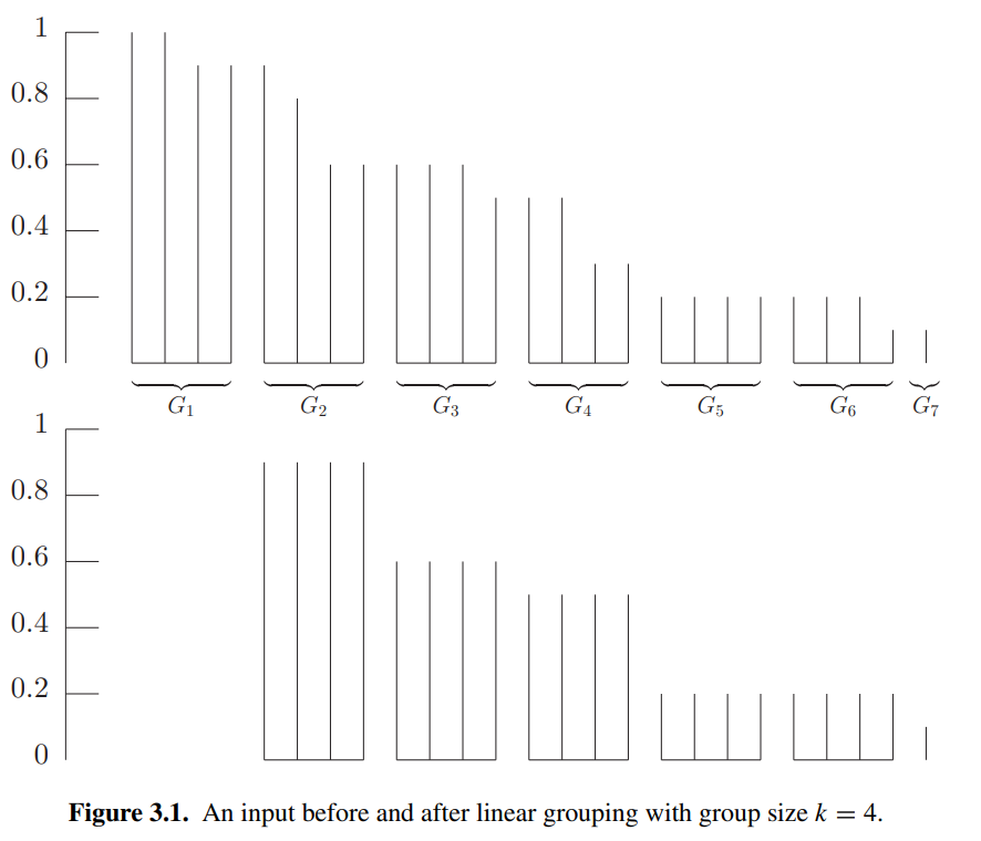
最后分析算法性能来设定 \(k\). \(I'\) 包含不同 size 的数量至多为 \(n / k\), 其中 \(n\) 是 \(I\) 中 piece 的数量,而 \(I\) 中去除了 small pieces, 从而 \(\mathrm{SIZE}(I) \geq \epsilon n / 2\). 令 \(k=\lfloor \epsilon \mathrm{SIZE}(I) \rfloor\), 于是 \(n / k \leq 2n / (\epsilon \mathrm{SIZE}(I)) \leq 4 / \epsilon^{2}\), 当 \(\epsilon \mathrm{SIZE}(I) < 1\) 时 large pieces 足够少可以直接 DP, 因此这里假定了 \(\epsilon \mathrm{SIZE}(I) \geq 1\). 再结合 Lemma 3.10, 最终的 bin 数量不会超过 \((1+\epsilon)\mathrm{OPT}(I) + 1\).
Theorem 3.12
For any \(\epsilon > 0\), there is a polynomial-time algorithm for the bin-packing problem that computes a solution with at most \((1+\epsilon)\mathrm{OPT}(I)+1\) bins; that is, there is an APTAS for the bin-packing problem.
-
Wikipedia 上的解释: Pseudo-polynomial time. ↩